Linear function and its graph

In the previous lessons we studied a linear equation with two variables, an equation of the form , . We found out that the graph of this equation is a line. Let's look at an example:

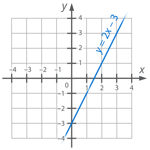
Example 1:

 (1)

Let's rewrite it so that Y is in one part and everything else is in the other part:

Let's reduce by 2:

Let's move y to the left side and everything else to the right:

 (2)

We obtained a special case of equation 1, in which Y stands alone in the left part; the graph of both expressions will be the same straight line, but we will call the entry 2 a linear function of Y from X.

Let us construct a graph of this function by making a table:

Define a linear function in the general case from a linear equation with two variables:

Since  we can divide both parts by b:

Let us introduce a more convenient notation:

,

We get the expression:

 (3)

For example №1 ,

Thus, a pair of numbers k and m defines a particular linear function.

In a linear function, the variable x is called the independent variable or argument of the function; we can choose an arbitrary value of x and use it to find the corresponding value of y.

Y is called the dependent variable or function.

A linear function is characterized by the fact that if the value of x is given, you can immediately get the value of y. y is a linear function of x.

Let us find the points of intersection with the axes for the linear function in general form (3). All points on the y-axis are characterized by the fact that their abscissa, the x-coordinate, is zero.

, ;

Point of intersection with the y-axis: (0, m)

Hence the geometric meaning of the variable m is the ordinate of the point of intersection of line 3 with the y-axis. The parameter m uniquely defines the point of intersection of line 3 with the ordinate axis.

The parameter  is called the angle coefficient.

All points on the x-axis are characterized by the fact that their ordinate is zero. Find the intersection point of our function with the x-axis:

, , ,

Point of intersection with the x-axis: ()

Example 2:

Plot the graphs of two linear functions:  (4),  (5)

In function 4 

In function 5 

In order to construct the graphs, we make tables in which we write the points of their intersection with the coordinate axes:

Table for function 4;

Table for function 5;

Fig. 2. Graphs of the functions y=-x+3 and y=x+3

So from the construction we see that when  (line ) the angle  between the line and the positive direction of the x-axis is acute, and when  (line ) the angle  between the line and the positive direction of the x-axis is obtuse.

The root of function 4 is -3, because at this value of x the function turns to zero.

The root of function 5 is 3, because at this value of x the function turns to zero.

Note that the solution of the following system:

is the point (0; 3).

Solving typical problems

Example 3 - find k and m:

We set a linear equation, since x and y are in the first power, with two variables.

To find k and m, perform transformations:

Let us write the resulting expression in the standard form:

It is obvious from this that , and 

Example 4 - find k and m:

Convert the right part:

Let us write the resulting expression in the standard form:

It is obvious from this that , and 

So, one of the standard problems is to find the parameters of a linear function k and m from a given linear equation.

Two more standard problems are to find y by a given value of x and vice versa, to find x by a given value of y. Consider an example.

Example 5 - Find the value of y at :

Such a problem is sometimes called a direct problem.

Example 6 - find the value of an argument if  :

This problem is called an inverse problem.

Lesson Conclusions

Conclusion: In this lesson we have looked at linear functions both in particular cases and in general, defined the parameters of a linear function and their meaning, introduced some new terms, and learned how to solve elementary typical problems.