A reminder of the theory from previous lessons, formulating the concept of direct proportionality
Recall that we are studying a linear equation with respect to two variables, x and y, an equation of the form ![]() ,
, ![]()
We know that the graph of a given equation is a straight line, each point of which is characterized by two numbers-coordinates x and y-the abscissa and ordinate, and each point satisfies a given equation.
In one of our lessons, we expressed y through x:
![]()
Using the fact that ![]() we can divide both parts of the equation by it:
we can divide both parts of the equation by it:
![]()
For convenience we took the following notations: ![]()
![]() , we get:
, we get:
![]()
Thus, we obtained a linear function y from x in general form. We introduced some new notations: x is called the independent variable or argument, y is called the dependent variable or function. k and m are parameters that completely and uniquely define a particular linear function.
Consider the special case of a linear function when ![]() , in this case
, in this case ![]() . This function is called direct proportion. It is defined by a single parameter k. We should study the effect of this parameter on the graph of the direct proportion function and on the function itself.
. This function is called direct proportion. It is defined by a single parameter k. We should study the effect of this parameter on the graph of the direct proportion function and on the function itself.
Example 1:
Let it be known that a hiker moves at a speed of 2 km/h from some point A to another point B. In this case the path he has traveled will obey the law:
![]() (1)
(1)
If it is known that a passenger rides the train from some point A to another point B, and the train moves at a speed of 60 km/h, then at any given time we can determine the distance of the passenger from the starting point by the formula:
![]() (2)
(2)
In general terms, both of these formulas can be represented as ![]() . It does not matter what the variables x and y imply, it only matters that one of them is independent, such as time, and the other is dependent, such as distance.
. It does not matter what the variables x and y imply, it only matters that one of them is independent, such as time, and the other is dependent, such as distance.
Let us return to our examples. In general terms, formulas 1 and 2 can be represented as
![]()
Hence, ![]() is one of the physical interpretations of the angle coefficient.
is one of the physical interpretations of the angle coefficient.
If we go to the formula of direct proportionality, then
![]()
Example 2:
![]() and
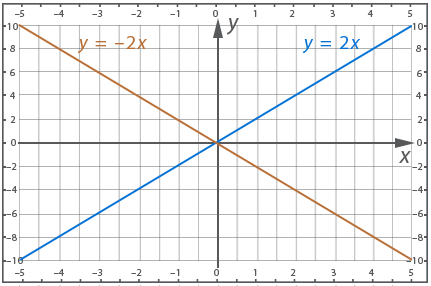
and ![]() - both functions are direct proportionality. Let's plot the graphs of these functions by making tables:
- both functions are direct proportionality. Let's plot the graphs of these functions by making tables:
|
х |
0 |
1 |
|
y |
0 |
2 |
Table for function 3;
![]()
|
х |
0 |
1 |
|
y |
0 |
-2 |
Table for function 4;
![]()
The coefficient of angularity is analogous to velocity in uniform rectilinear motion.
One of the main tasks is to be able to find the angular coefficient in various expressions.
Example 3 - find the angle coefficient:
![]()
![]()
It is obvious from this that ![]()
![]()
![]()
It is obvious from this that ![]()
Note also that if k < 0, the angle between the function graph and the positive direction of the x-axis is blunt and the function decreases, and if k > 0, the angle is sharp and the function increases, as can be seen in the graph in Example 2.
The physical analogy is this: if a hiker has left home and his speed is 2km/h, then at each moment the distance from him to home increases, and if we say that the distance is expressed as ![]() , it means that he returns home and the distance decreases.
, it means that he returns home and the distance decreases.
Formulation of the properties of this function
Let us formulate the properties of direct proportion:
- The graph of any such line passes through the origin of coordinates, since in the equation ![]() at
at ![]() regardless of the value of
regardless of the value of ![]() - Y will be equal to zero;
- Y will be equal to zero;
- Let's look at a few functions:
![]() - direct proportion;
- direct proportion;
![]() - linear function;
- linear function;
![]() - linear function;
- linear function;
Construct the graphs of these functions. Each of them has ![]() . The first has
. The first has ![]() , the second has
, the second has ![]() , the third has
, the third has ![]() . Recall that the parameters k and m are determined from the standard linear equation
. Recall that the parameters k and m are determined from the standard linear equation ![]()
Let's make tables for graphing:
|
х |
0 |
1 |
|
y |
0 |
2 |
Table for the first function;
|
х |
0 |
-0.5 |
|
y |
1 |
0 |
Table for the second function;
|
х |
0 |
0.5 |
|
y |
-1 |
0 |
Table for the third function;
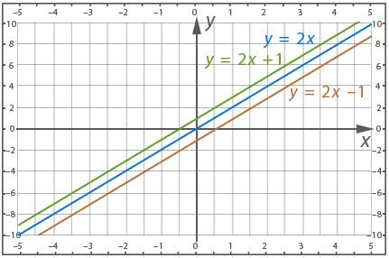
As we see, the constructed lines are parallel, the reason for this is the equality of their angular coefficients. There is a theorem that states:
If ![]() is a graph of direct proportionality, then the graph of
is a graph of direct proportionality, then the graph of ![]() will be parallel to it, because the coefficient k determines the angle of slope to the x-axis, and this coefficient of the functions is equal.
will be parallel to it, because the coefficient k determines the angle of slope to the x-axis, and this coefficient of the functions is equal.
Example 4 - plot graphs of functions:
![]()
![]()
![]()
![]()
Immediately note that the lines will not be parallel, since their angular coefficients are not equal.
To construct each graph, it is enough for us to choose one point, since the second point is already known - it is the point (0; 0).
So, for the first graph we take the point (1; 1)
For the second graph take the point (1; 2)
For the third graph (1; -1)
For the fourth graph (1; -2)
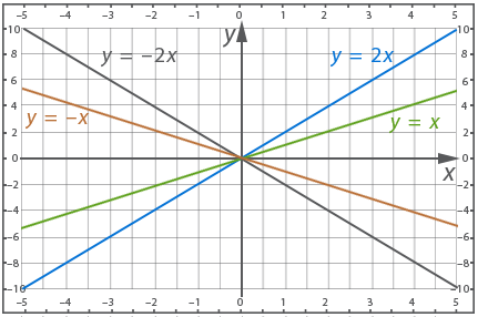
You can see very well from the graph that straight line ![]() went steeper than straight line
went steeper than straight line ![]() , the angle of straight line
, the angle of straight line ![]() is less sharp, with the same values of the argument the value of the function
is less sharp, with the same values of the argument the value of the function ![]() is greater than
is greater than ![]() , but in both cases the angle is sharp and the function is increasing.
, but in both cases the angle is sharp and the function is increasing.
Both lines ![]() and
and ![]() have an obtuse angle and both functions decrease, but line
have an obtuse angle and both functions decrease, but line ![]() is less obtuse and this function decreases faster.
is less obtuse and this function decreases faster.
Example 5 - determine the relationship between the angle coefficients:
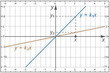
![]()
![]()
![]() from here
from here ![]()
So, the role of the angle coefficient is the rate of growth of the function.
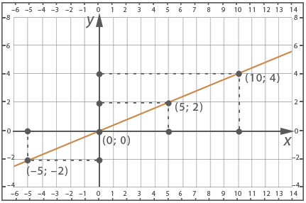
Example 6:
Construct a graph of a straight line if it is known to belong to the point with coordinates (2; 8)
We need two points to draw the line, the first of which is (0; 0), since all graphs of a direct proportion go through the point (0; 0), and the second point is given, which is the point (2; 8).
We can do things differently. From a given point (2; 8) we understand that x=2 and y=8 satisfy our equation of the form ![]() , substitute these values and find k:
, substitute these values and find k:
![]() , from here
, from here ![]() . So we are given an equation
. So we are given an equation ![]() , which we can easily construct.
, which we can easily construct.
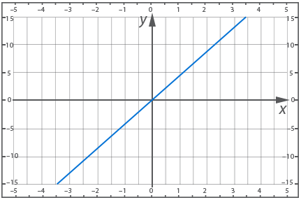
Example 7:
Construct a graph of the direct proportion of ![]() and use it to answer many questions.
and use it to answer many questions.
Let's start by constructing the graph. We know the first point - for any graph of a straight line it is the point (0; 0). For the second point, take ![]() , then
, then ![]() :
:
From the graph determine the value of the function for the following values of the argument: ![]() ,
, ![]() ,
, ![]() ,
, ![]() ;
;
In addition, from a given value of the function determine the value of the argument:![]()
![]() ,
, ![]() ,
, ![]()
Determine from the graph the solution to the inequalities:
![]() и
и ![]()
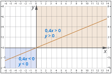
y<0 at x<0
y>0 at x>0
Example 8 - find the largest and smallest values of a function, if they exist:
1) The function ![]() is given, and
is given, and ![]()
2)![]() ,
, ![]()
Let's graph the function ![]() :
:
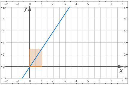
For the first case x varies within ![]() , so y varies within
, so y varies within ![]() , so on this interval the minimum of the function is zero, and the maximum is three.
, so on this interval the minimum of the function is zero, and the maximum is three.
For the second case, x varies within ![]() , so the function varies within
, so the function varies within ![]() , which means that the minimum value of the function on this interval exists and is equal to three, and the maximum value of the function is not reached.
, which means that the minimum value of the function on this interval exists and is equal to three, and the maximum value of the function is not reached.
The last type of problem is to determine the angle coefficient from a given graph.
Example 9 - Determine the angular coefficient:
A graph of a direct proportion is given.
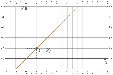
We see that the graph passes through point (1; 2), so the pair of numbers x=1, y=2 satisfies a function of type ![]() , so we can substitute the values in the equation and find k:
, so we can substitute the values in the equation and find k:
![]()
So we have a graph of the function ![]()
Lesson Conclusions
Conclusion: In this lesson we have considered a special case of a linear function - direct proportion. We have formulated properties of this function and basic typical problems related to this topic.
2. If you find an error or inaccuracy, please describe it.
3. Positive feedback is welcome.